Prerequisite Math: Calculus
Prerequisite Coding: Python (Tensorflow)
Introduction
Most of today’s state-of-the-art machine learning models are some kind of deep neural network. But while such models are excellent at fitting complex functions to model relationships between features (X) and targets (y), one of their biggest downsides is that they can take a very long time to train. There are several ways you can mitigate this such as (this list is not exhaustive):
- Weight Initialization (e.g. Glorot-He Initialization)
- Non-saturating activation functions (e.g. ReLU)
- Batch or Layer Normalization
- Pretraining (particularly in the NLP setting)
I encourage you to experiment with as many of these hyperparameters as possible to see what works best. However in this post, I’m going to talk about one of the biggest ways to improve training time: the optimizer. Most deep learning frameworks (and indeed many non-neural modelling solutions) use some version of Gradient Descent as the default optimizer. While this is an excellent way to generate optimal weights in your network, researchers have in the past decade or so, come up with a variety of clever ways to modify this procedure to ensure faster and smoother convergence than is typically found in SGD. Specifically, I’m going to walk you through the following alternative procedures:
- Momentum
- Nesterov Accelerated Gradient
- AdaGrad
- RMSProp
- Adam
- Nadam
We’ll discuss how each of these is computed, as well as the intuition behind them. Then we’ll train a fixed model, and visualize how some of them work faster than traditional gradient descent.
Review of SGD
Gradient Descent is an iterative optimization algorithm that is designed to find the minimum of a surface by repeatedly taking steps in the opposite direction of the direction of steepest increase. By definition, the direction of greatest increase at a point on a surface is the gradient, or the vector of partial derivatives evaluated at that point. For example, if the surface is given by the function \( f = 5x^2 + 2xy + 3y^2 \), then the gradient is given by \( \nabla_{f} = [ \frac{\partial f}{\partial x}, \frac{\partial f}{\partial y} ]^T = [10x +2y , 2x + 6y] \). If we’re at a specific point, say \( (x = 1, y = 1)\), then the gradient has real entries, \([12, 8]^T \).
Most neural networks update weights (and biases) according to the following formula:
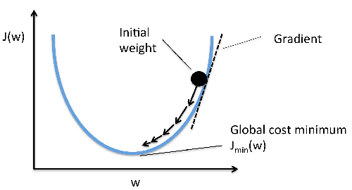
\[w := w - \alpha \frac{\partial L}{\partial w}\]Where \( w \) typically denotes the weight matrix. Doing this for a number of epochs will usually result in convergence to the minimum of the loss function (ie the weights converge to their optimal values). The following graph shows this process of iteratively descending the loss surface until the optimal weights are found. I’d also like to mention that I never claimed to be an artist:

In the formula above, \( \alpha \) denotes the learning rate, which is a hyperparameter designed to control step size. You can see that eventually, repeated iterations of weight updates reach the globabl minimum of the loss function. The dotted lines represent the gradients at fixed points along the way. Notice also that we’re assuming the surface is differentiable (and continuous) for the entire domain of weights. However, the loss function does not necessarily have to look ‘pretty’. There may be many local optima and saddle points in which regular GD can get stuck. Some of the technique’s we’ll discuss shortly are also great at avoiding this problem.
One final thing I’d like to mention is that Gradient descent is considered a first-order optimization algorithm, because we only ever work with the first derivatives of the loss surface. Although higher-order derivatives may work well in theory, in practice, this involves computing the Hessian (matrix of second derivatives) of the loss, which for an entire matrix containing millions of weights, involves far too many parameters to be feasible in practice. In future I may dedicate a separate post to higher-order optimization methods, but for now just know that they do exist (and they’re a fascinating area of research).
Momentum
For those familiar with Newtonian physics, momentum measures the quantity of motion of an object. It is computed as the product of an object’s mass and velocity, and it is this physical interpretation that inspired the Momentum Optimization variant. Regular Gradient descent does not care about the gradients in previous update iterations - if the current value is small, so will be the update. This can sometimes cause convergence to take a very long time. Conversely, Momentum optimization cares a lot about earlier gradients. At each iteration, instead of subtracting the gradient directly, it subtracts the gradient from a momentum vector, and updates the weights by adding the momentum vector to the previous instance. Here are the equations defining Momentum:
\[V_{w} := \beta V_{w} + (1 - \beta) \nabla_{w} J(w)\] \[w := w - \alpha V_{w}\]There would be identical equations for updating the bias term as well. Notice that we now have an additional hyperparameter: \( \beta \in (0,1) \). This is called the momentum parameter. You can think of this new term as a friction mechanism: when small, there is little momentum, and the update is controlled almost exclusively by the gradient. However, when the momentum coefficient is large, the optimizer moves very quickly towards the minimum. In practice, it is common to set \( \beta = 0.9 \). We want a good deal of friction, otherwise the optimizer will quickly reach the minimum, but will overshoot it, continuing to oscilate and taking longer than we would like.
A couple of other things to note. Often in the literature, you will see the first equation written as \( V_{w} := \beta V_{w} + \nabla_{w} J(w) \), which has the effect of scaling the equation by \( 1 - \beta \), but the principle is identical. Also, some papers don’t bother using this on the bias term. Notice too that in these equations, the gradient acts not as the velocity, but as the acceleration ( \( V_{w} \) is akin to the velocity). If there is a drawback in using Momentum, it’s that you now have another hyperparameter to tune (yay!). However in certain situations, such as when there is no batch normalization, and features can have very different units, this addition can save a lot of time.
So how do we implement this in Tensorflow? Luckily, it’s incredibly easy. There’s a built-in hyperparameter for including it in the optimizer:
optimizer = keras.optimizers.SGD(learning_rate = 0.02, momentum = 0.9)
Nesterov Accelerated Gradient
This method just involves a small variation on momentum, but it almost always works even faster. All we do to adapt momentum into Nesterov’s accelerated gradient is modify the gradient itself:
\[V_{w} := \beta V_{w} + (1 - \beta) \nabla_{w} J(w + \beta V_{w})\] \[w := w - \alpha V_{w}\]This might seem like a small change, but it can have very large performance gains. Why? Well now we’re measuring the gradient of the cost function not at the local weight position \( w \), but slightly ahead of it. Since the momentum vector is pointing in the direction of the optimum, it is more accurate to take steps in that direction instead of the direction of the local gradient. After many steps, these small improvements add up and this variation can be significantly faster.
Just like regular momentum, implementing this in Tensorflow is quite simple. We just set the Nesterov hyperparameter to True:
optimizer = keras.optimizers.SGD(learning_rate = 0.02, momentum = 0.9, nesterov=True)
This method was introduces by Yurii Nesterov in a paper in 1983 (i’ll include the original paper in the reading section), but it was first adapted to training deep neural networks in a paper by Ilya Sutskever et al in 2013. They gave it the name Nesterov Accelerated Gradient, or NAG, so you may see it referred to in this way.
AdaGrad
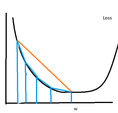
Suppose our loss function is shaped like an elongated bowl (this is true for small neighborhoods even if the global function is very ‘wiggly’). During the beginning of Gradient descent, the gradient will be pointed mostly downward, with only a small shift on the horizontal axis. This changes gradually in later steps, but overall, the path of descent towards the optimimum resemble something close to an ‘L’ shape, but with a rounded corner. What if instead of following this shape (vertical, then horizontal descent) we proceeded directly towards the optimum? Think about it like following the hypotenuse of the triangle. We could potentially save a lot of time. Here’s a picture showing what I mean:

You can see that going directly towards the minimum (the orange trajectory) would be much quicker than the blue trajectory (the distance would be shorter). This is exactly the idea behind the Adaptive Gradient, or AdaGrad method. We do this by scaling down the gradient in its steepest directions (which are usually closer to vertical than horizontal). Here are the update equations:
\[s \leftarrow s + \nabla_{w} J(w) \otimes \nabla_{w} J(w)\] \[w \leftarrow w - \alpha \nabla_{w} J(w) \oslash \sqrt{s + \epsilon}\]So what’s going on here? Well the first equation accumulates the squares of the weight gradients. This has the effect of identifying the steepest directions of the gradient, which will grow when squared (the directions that are not steep will not grow relative to their counterparts). Note that the \( \otimes \) symbol is called the Hadamard Product, and simply denotes elementwise multiplication. In the second equation, we update the weights, downscaling the original gradients by \( \sqrt{s + \epsilon} \) (note the special notation for elementwise division). Since s accumulated the square gradients, this has the effect of downscaling the steeper directions more than the others, leading to a descent that is oriented closer to the true optimum (avoiding the ‘L’ shape I discussed earlier). \( \epsilon \) is a smoothing parameter, added to prevent dividion by 0, and is typically set to 10e-10.
Overall, this algorithm decays the learning rate faster for steeper dimensions than for gentler ones. We call this an adaptive learning rate, and it requires much less tuning of the \( \alpha \) parameter than with other methods. An unfortunate downside of this technique is that although it is great for simple surfaces like linear regression, on neural nets it often stops too soon. The learning rate is downscaled so much that we never reach the minimum loss. There is a built-in AdaGrad optimzer in keras, but it rarely makes sense to use (though you could use it for simpler models, like regression). So why do I mention it? Well understanding why it works is key to understanding the next optimization technique.
RMSProp
To prevent the AdaGrad algorithm from stopping too soon, we accumulate only the gradients from recent iterations instead of all gradients since training began. To accomplish this, we use a setup similar to momentum, placing an exponential decay on our \( s \) vector:
\[s \leftarrow \beta s + (1 - \beta) \nabla_{w} J(w) \otimes \nabla_{w} J(w)\] \[w \leftarrow w - \alpha \nabla_{w} J(w) \oslash \sqrt{s + \epsilon}\]Only the first equation really changes. In practice, a value of 0.9 for \( beta \) tends to work quite well. Although this does add another hyperparameter, the default value tends to be near the best possible, so depending on the application, you may not actually have to tune it. Unless the problem is very simple, this Root Mean Squared Propagation (RMSProp) algorithm almost always outperforms AdaGrad. Note that this was invented by Hinton and his students, but was never formally published.
Implementing this in keras is, as you might expect, quite simple:
optimizer = keras.optimizers.RMSProp(learning_rate= 0.02, rho = 0.9)
In the above implementation, \( \beta \) is represented by the rho argument. To reiterate, using this will dampen the oscillations in descent and lead to faster convergence just like with AdaGrad, but we no longer have to worry about stopping too early. This algorithm was the preferred choice of researchers for a few years, until the next technique was introduced.
Adam
Adaptive Moment Estimation (Adam) combines the ideas of momentum and RMSprop. It keeps track of past gradients just like momentum, and it also keeps track of scaled squared gradients like RMSProp. There are several equations in this case, but we’ve covered them already:
\[m \leftarrow \beta_1 m - (1 - \beta_1) \nabla_{w} J(w)\] \[s \leftarrow \beta_2 s + (1 - \beta_2) \nabla_{w} J(w) \otimes \nabla_{w} J(w)\] \[\hat{m} \leftarrow \frac{m}{1 - \beta_{1}^{t}}\] \[\hat{s} \leftarrow \frac{s}{1 - \beta_{2}^{t}}\] \[w \leftarrow w - \alpha \hat{m} \oslash \sqrt{\hat{s} + \epsilon}\]In the equation above, \( t \) represents the iteration number, beginning at 1. You can see that this is very similar to both RMSProp and to Momentum. The third and forth equations are typically initialized at zero. Since they will be biased towards zero early in training, they help to boost \( m \) and \( s \). We now have several hyperparameters, but don’t worry. Typically in practice, \( \beta_1 \) is initialized to 0.9, and \( \beta_2 \) initialized to 0.999. The smoothing parameter is, as before, initialized to a small number like 10e-0.7. Finally because Adam is an adaptive method, you don’t need to worry as much about tuning the learning rate (0.001 usually works well).
Why moment estimation? Well these equations are estimating the mean and variance of our gradients, which are also called the first and second moments. And like our other methods, this one is also easy to implement in Keras.
optimizer = keras.optimizers.Adam(learning_rate = 0.001, beta_1 = 0.9, beta_2 = 0.999)
Note that the smoothing parameter will default to None, which will direct keras to use the keras.backend.epsilon() parameter, which defaults to 10e-07.
Nadam
- Nadam optimization is exactly what you’re thinking: Adam optimization combined with the Nesterov trick. Now the gradient is not evaluated at the local point, but is instead evaluated at the sum of the local weight and current momentum:
Often this variation converges slightly faster than Adam. However, the paper introducing this technique finds that sometimes RMSProp can outperform Nadam. So it is wise to try several different optimizers for your task, to see which one works best. Just as a caveat, current research has found that although adaptive methods like RMSProp and Nadam can greatly improve training speed, in some cases they can lead to models that do not generalize very well. In these cases you may be better off using a slower optimization to achieve a higher test error. Or try using regular Nesterov Accelerated Gradient instead of these more complex optimizers.
Application
Now let’s actually test some of these optimizers. This is relatively easy to do in Keras, since the loss history can be easily extracted from a trained model. The data i’ll use is the built-in fashion MNIST dataset found in the keras datasets library. It consists of 70,000 grayscale 28 x 28 images, which I will split into train and test sets. I’m also going to scale the pixel values to be between 0 and 1 (this helps training). I use a train test split of 60000, 10000. Note that in this case, I don’t really care much about overall performance - I’m just trying to demonstrate the differences in optimizers.
from tensorflow import keras
# 70000 grayscale 28 x 28 images, 10 classes
fashion_mnist = keras.datasets.fashion_mnist
from time import time
import matplotlib.pyplot as plt

(X_train_full, y_train_full), (X_test_full, y_test_full) = fashion_mnist.load_data()

# Scale
X_train_full, X_test_full = X_train_full/255.0, X_test_full/255.0
y_train_full, y_test_full = y_train_full, y_test_full

class_names = ["T-shirt/top", "Trouser", "Pullover", "Dress", "Coat",
               "Sandal", "Shirt", "Sneaker", "Bag", "Ankle boot"]
Now I’ll define a simple feed forward network. First I flatten the images into a single column vector, then I pass that input through a couple of dense layers. It’s fairly self-explanatory. Ultimately our output will be a softmax score over 10 classes (see the categories listed above).
model = keras.models.Sequential([
  keras.layers.Flatten(input_shape=[28,28])), # same as X.reshape(-1,1)
  keras.layers.Dense(300, activation = "relu"),
  keras.layers.Dense(100, activation = "relu"),
  keras.layers.Dense(10, activation = "softmax")
  ])
Now I’ll compile and fit the model first using regular SGD. I’ll also time the fit method:
model.compile(loss="sparse_categorical_crossentropy",
              optimizer="sgd",
              metrics=["accuracy"])
sgd_start = time()
sgd_history = model.fit(X_train_full, y_train_full, epochs = 15,
                        validation_data = (X_test_full, y_test_full))
sgd_end = time()
sgd_time = sgd_end - sgd_start
This may take a few minutes to run, but once it has, we can quickly extract the validation loss for each iteration (i’ve chosen 30 epochs somewhat arbitrarily, but feel free to fiddle with that number as long as you keep in constant across optimizers). Next let’s retrain the model using Nadam:
# Nadam
model.compile(loss="sparse_categorical_crossentropy",
              optimizer=keras.optimizers.Nadam(beta_1 = 0.9, beta_2 = 0.999),
              metrics=["accuracy"])
nadam_start = time()
nadam_history = model.fit(X_train_full, y_train_full, epochs = 15,
                        validation_data = (X_test_full, y_test_full))
nadam_end = time()
nadam_time = nadam_end - nadam_start
Lastly, let’s run RMSProp. In each of these cases, I use the default hyperparameter values we discussed earlier.
# RMSProp
model.compile(loss="sparse_categorical_crossentropy",
              optimizer=keras.optimizers.RMSprop(rho = 0.9),
              metrics=["accuracy"])
rmsp_start = time()
rmsp_history = model.fit(X_train_full, y_train_full, epochs = 15,
                        validation_data = (X_test_full, y_test_full))
rmsp_end = time()
rmsp_time = rmsp_end - rmsp_start
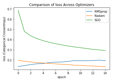
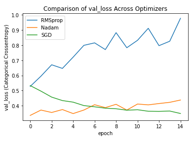
Lastly I’ll show you the loss functions (train and val) for each of these optimizers:
def plot_loss(history_metric):
  plt.plot(range(15), rmsp_history.history[history_metric], label = 'RMSprop')
  plt.plot(range(15), nadam_history.history[history_metric], label = 'Nadam')
  plt.plot(range(15), sgd_history.history[history_metric], label = 'SGD')

  plt.title('Comparison of {} Across Optimizers'.format(history_metric))
  plt.xlabel('epoch')
  plt.ylabel('{} (Categorical Crossentropy)'.format(history_metric))
  plt.legend()
  plt.show()

plot_loss('loss')
plot_loss('val_loss')
Here are plots showing the resulting loss and validation loss. Admittedly there is some overfitting going on here, but notice how quickly Nadam and RMS prop get to low levels of loss both in training and validation. This can save quite some time on larger datasets.


Now this was a very general demonstration. The effects are likely even more extreme when the hyperparameters are properly tuned (in particular the learning rate). I encourage you to do this.
Conclusion
We’ve covered a lot of information today, but the key takeaway is that there are way more powerful optimization methods than regular Gradient Descent. Note that many of these optimizers will produce very dense models (lots of nonzero parameters), which can slow down your training time. To avoid this, you might try using L1 regularization. There are also several open-source packages designed to speed up tensorflow model training.
Most people do not imagine optimizer choice to be a hyperparameter. But while it is true that certain optimizers generally outperform others, I encourage you (whenever you have time) to try a variety of them on every ML task.
Further Reading
-
Here is the original Nesterov paper: A Method for Unconstrained Convex Minimization Problem with the Rate of Convergence \( O(1/k^2)\). Yurii Nesterov. Doklady AN USSR 269 (1983): 543-547.
-
Here is the NAG paper: On the importance of initialization and momentum in deep learning. Ilya Sutskever, James Martens, George Dahl, Geoffrey Hinton ; Proceedings of the 30th International Conference on Machine Learning, PMLR 28(3):1139-1147, 2013.
-
Here is the AdaGrad paper: Adaptive Subgradient Methods for Online Learning and Stochastic Optimization. John Duchi et al., Journal of Machine Learning Research 12(2011): 2121-2159.
-
Here is the Adam paper: _Adam: A Method for Stochastic Optimization._Diederik P. Kingma and Jimmy Ba. arXiv preprint: 1412.6980 (2014)
-
Here is a great article by Jason Brownlee that builds Nesterov Momentum from scratch.
-
The Keras optimizers documentation is quite helpful too.